Mechanical motion

Terms view on Wikipedia.

Introduction

Computational physics large wide use to modern scientific research.
However, models of computational physics are not simulation models. The simulation model reproduces the message exchange protocol between the components of the system under study. Somewhat simplifying, we can say that the simulation model and the object of study should have the same behavioral algorithm. The numerical model reproduces operations with numbers and, in general, modeling mathematical object. For example, solving the equations of Newton’s motion, the numerical model reproduces not the motion of a point particle, but the process of solving a differential equation. In this way, where is a problem of development of physical simulation models. You can object, in physics have been created many qualitative mathematical models, modern numerical methods are effective, and researcher no need to other approaches. With it we can argue - a new approach always eventually gives something new.

In this section, we shall discuss simulation in physics.The simulation model of classical mechanical motion was propose in papers [1-3]. This model based on the Levi-Beck theory of mechanical motion in discrete space-time.

Related Works

There are works on simulation modeling in physics but they are few and most part are case studies. These works cannot compete with works of performed in a traditional manner of research. There is a problem of an adequate description of physical processes in the language of simulation modeling. In the book [4] this approach is called algorithmic or constructive physics. Similar views are held by the authors of the book [5]. This problem is closely related to the problems of digital physics [6] (see digital mechanics book) and the methods of information physics [7].
Our approach relies heavily on the works of Stefon Wolfram [9] and Gerard ‘t Hooft [10].

Problem Domain

Newton’s laws

• First law: In an inertial frame of reference, an object either remains at rest or continues to move at a constant velocity, unless acted upon by a force.
• Second law: In an inertial reference frame, the vector sum of the forces F on an object is equal to the mass m of that object multiplied by the acceleration a of the object: F = ma.
• Third law: When one body exerts a force on a second body, the second body simultaneously exerts a force equal in magnitude and opposite in direction on the first body.

More info view on Wikipedia.

Analysis model

Fundamentals of mechanical motion in discrete space-time were developed in the period of the birth of quantum mechanics [8]. In our opinion, these views can become a theoretical basis for constructing simulation models. We will not discuss the question of the discreteness of physical space. Our task is to find ways to adequately describe the mechanical motion by means of simulation modeling.

In our model, we use a two-layer architecture (see Fig. 1), which allows us to separate the components of the model into two levels of abstraction. The lower layer defines abstract model classes (see Figure 3), such as Component, Composite, and ListItem. The ReusableClassesOfInterface package contains abstract classes modeling the research installation and the user interface libraries (we use VCL). Top-layer packages define specific classes, such as ConcreteTreeNode, TreeLeaf, TreeRoot, and classes of a specific simulation model. In UML2 SP, an architectural diagram in terms of subject semantics is an interpreted as a conceptual graph.

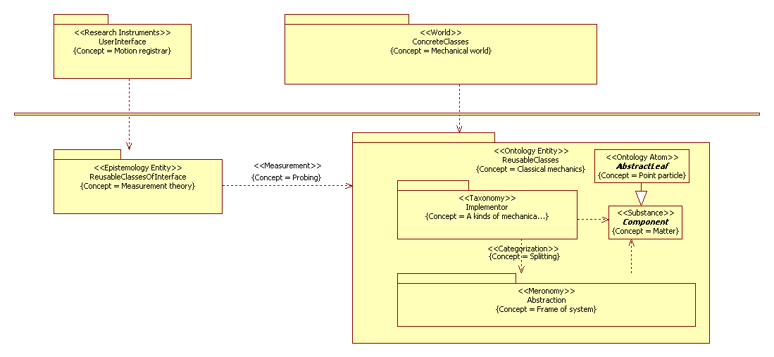
Figure 1. Architecture of the simulation model

Package «Epistemology Entity». This package defines the procedure for measuring the main characteristics of the mechanical movement - time, position, speed and acceleration. Both packages «Epistemology Entity» and «Research Instruments» named Epistemology partition.
Package «Ontology Entity». This package has the marked meaning “Classical mechanics” in the sense that by theory we mean the classification of mechanical systems. Both packages «Ontology Entity» and «World» named Ontology partition.

1. Ontology partition

A conceptual model in UML2 SP is an analysis class diagram. This diagram considered as ontology. Model a mechanical motion is depicted in Fig.2.

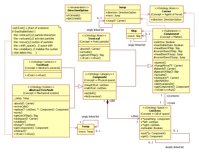
Figure 2. The class diagram

Description of a computational semantics

All objects of Component class have concurrent threads.

Description of an application domain semantics

We shall give definition of concepts to the ontology. The architecture of the model defines the pattern Composite, which defines the hierarchy of nested mechanical subsystems. Unlike the classic pattern, aggregation materializes through a linked list with ListItem elements.

Matter

The “Component” frame define “Matter” concept. In the classical physics, matter is any substance that has mass and takes up space by having volume. The frame has “headItemOfJump” and “currentItemOfJump” slots. It is define “Resource of motion” concept. The frame has “headItemOfSkip” and “currentItemOfSkip” slots. It is define “The inertial mass” concept. The property of body is called inertia. A quantitative measure of inertia is mass.
The doImpact() method define “Influence” concept. The concept describes to act of force to body and change value headItemOfJump slot.
Newton’s second law. In 1926, Levi proposed the following mechanism action of force [8, P.98]. The force acts on the particle not constantly, but every τ sec (τ ~ E-23 sec). On any other particle, whose mass is N times larger, the force acts every Nτ sec.
We use the Carrier class such that generates new instances of the headItemOfJump list. The Component class has both headItemOfSkip and currentItemOfSkip fields of type Skip. This list simulates the inertia of a particle when skips objects of Carrier. A quantity of skip is quantity elements in the headItemOfSkip list (see Fig.3). If ‘currentItemOfSkip’ list end then object of Carrier is processed. The changeMove() method change length of the list. The absorb() method change a state of object Carrier class. The getListOfSkip() method return a pointer headItemOfSkip. Both methods absorb() and getListOfSkip() are abstract methods and shall be must define in a concrete class. A detailed of algorithmic record of Newton’s 2nd law is discussed in [2].

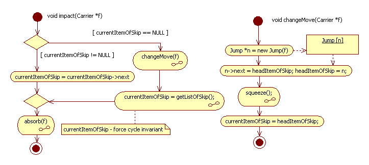
Figure 3. Algorithmic recording of Newton’s second law

Point particle

The “TreeLeaf” frame define “Point particle” concept. A point particle is an appropriate representation of any object whose size, shape, and structure is irrelevant in a given context. The TreeLeaf class define both methods absorb() and getListOfSkip(). The absorb() method change direction of Carrier to the contrary. It is action of particle to the carrier of force. The getListOfSkip() method return a pointer headItemOfSkip. The «Exist»Run() method define rule of change of isActive value.

void Run(){
		if (currentItemOfJump->next != NULL) {
		if (currentItemOfJump != NULL) {
			currentItemOfJump = currentItemOfJump->next;
		} else {isActive = false;};
	}

If isActive is false then particle do not can motion (see below Newton’s first law). The actuate() method make particle is the active

	void actuate() {
	if (headItemOfJump != NULL) {isActive = true; };
	currentItemOfJump = headItemOfJump;
	}

Agent of force

The “Carrier” frame define “Agent of force” concept. Agent of force is a carrier of interaction. The frame has «Direction» slot. In 1-dimension space, it is field can has two value are backward and forward.

Cell of space

The “ListItem” frame define “Cell of space” concept. The frame has “left” and “right” slots. It is defined “coupling” (or “topology”) notion. The frame has “something” slot. It is define “content” notion. The cell of space do not material object (do not daughter of Component class).

Physical space

The “Composite” frame define “Physical space” concept. Physical space has the base point and the anchor points. The base (the headOfList attribute) and the anchor points (tailOfList attribute) specify the direction in the physical space. From the point of view of computational semantics, space is an N-dimensional linked list of instances of the ListItem class. The space assembly is

for (int i = 0; i < 1000; i++) m[i] = NULL;
	
	for (int i = 0; i < N; i++) { // N - resolution of space
		m[i] = new ListItem; m[i]->x = i;
	};
	ListItem *a;
	for (int i = 0; i < N; i++) {
	a = m[i];
	if (i<N-1) a->right = m[i+1]; if (i>0) a->left = m[i-1];
	};
	headOfList = m[1];    // base of space
	tailOfList = m[N-1];  // anchor point 

Further, we confine ourselves to a one-dimensional space. The listShift() and listInversion() method are operations above space.

Mechanical system

The “AbstractTreeNode” frame define “Mechanical system” concept. This class defines abstract operation Run(). The «Exist»Run() method is

	void Run() { //  ** quantum of existence of the system

if (hasStableState) {
this->interact();  // ** particles interaction
this->actuate();   // ** activate particles
this->move(); // ** displacement of point particles
this->listShift();  // movement of the system
this->Stabilize();
} else { ShowMessage("decay "+frame->Caption);
		delete this;
		 };

The interaction() method define particles interaction. It method is abstract method and must defined to concrete classes. For this method defined constraint.
Newton’s third law. This law is specified as a constraint: the doImpact() method can only be used in pairs. For example, the following pair of interactions

f = p-> doImpact (f); // p - the point particle 
f = headOfList-> something-> doImpact(f); // massive body

The move() method define a motion of particles.
Newton’s first law. To solve the isotachy problem, we used a somewhat modified theory of mechanical motion in discrete space-time, proposed by Beck in 1929 [8, P.28]. The essence of this theory is as follows. A moving point particle has some stock of motion, which in our case is modeling by a linked list from Jump instances. The faster particles have a longer list. The move() method of the AbstractTreeNode class executes a single jump (replace (b, p) method), after which the list is reduced by one position (the «Exist»Run() method of the TreeLeaf class). If the list is exhausted, the particle is deactivating and will no longer move. The move() method is called many times, so that all the particles finish moving. The call loop is organized as a linked list of the Temp class instances. In detail, this mechanism is discuses in [1].

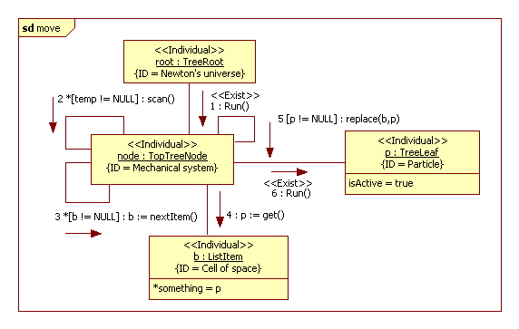
Figure 4. Activity move()

The doImpact() method.
The doImpact() method simulate act of external force to mechanical system and call absorb() and getListOfSkip() methods. Both methods are abstract methods. The absorb() method simulate deformation of system and defined to concrete classes. The AbstractTreeNode partly define doImpact() method. It is getListOfSkip() method. The getListOfSkip() method return mass of mechanical system and expresses property of additivity of mass.

The Newton three laws must supplement by yet two propositions.
Collision. To resolve the collision situation, in the AbstractTreeNode class (in replace (b, p) method) defined the bump() method . The method is virtual and can substitute in descendants of the AbstractTreeNode class. If a method of the AbstractTreeNode class is caused by then it is an absolutely elastic collision.
Disintegration. The AbstractTreeNode class defines a private field hasStableState. If this field is false, the system self-destructs. This field can be changed by the procedure stabilize(), which can be substituted in descendants of the AbstractTreeNode class. If the AbstractTreeNode method is caused by then the field is set to true.

Newton’s universe

The “TreeRoot” frame define “Newton’s universe” concept. The TreeRoot class specifies the initial and boundary conditions.

2. Epistemology partition

1. Tools of measurement

The measurement procedure include a controlled violation of class encapsulation. The model of the measuring system is a depicted in Fig.5.

One of the most effective methods of studying space is the lattice method, which is an analog of Cartesian coordinates method. The essence of the method is to map the space to an array of the appropriate dimension, and to make measurements using an array. The mapping must updated at each step of the time In Fig.5, the Subject class simulate a reference frame. The Subject class has an array of rf pointers of type Item. The model of the measuring device create based on the Observer pattern. The Notify() method of the Subject class is called from the «Exist»Run() method of the AbstractTreeNode class after all mechanical processes are completed.

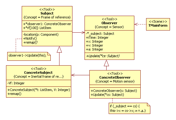
Figure 5. Model of measuring system

Specific ConcreteSubject classes define reference frames (RF) of different kinds, for example, inertial reference frames (IRF), non-inertial RF (NRF), frames with non-card coordinates, etc. Next, we will mainly use IRF.

2. Natural and standard units of measurement

Measurements in discrete models are much more convenient to carry out in natural units of measurement. Let us give the formulas for the conversion of natural units of measure to standard ones and back. The basic units of measurement in the CGS are centimeter, gram, and second. Let l [cm] = l’/λ, m [g] = m’/μ, t [s] = t’/τ, where the natural units of measurement (dashed) are measured in the number of instances of the Item, Skip and number of cycles Exist. The case of a unit mass corresponds to a situation where the list of instances of Skip is empty (that is, particles with 0 mass do not exist). The triple of numbers (λ, μ, τ) will called the resolution of the model.
Consider the derived units. The speed is expressed in the number of v’ instances of the Jump class in the motion amount list; v [cm/s] = (τ/λ)v’ or v’ = (λ/τ)v. Acceleration is also expressed in the number of a’ instances of the Jump class, because this is the difference of the two lists of momentum; a[cm/s2] = a’ х τ²/λ. Force is the quantity of F’ acts of interaction: F[dyne, g • cm/s²] = ma = m’/μ х (τ²/λ)a’ = τ²/(μλ) х F’. The conversion factor can be fractional; to give a physical meaning to such coefficients, the ratio must multiplied by a certain power of 10. Energy and work in natural units are measured in the number of acts of work. The act of work is a single movement of a particle from one cell to another with a single act of interaction. The work A [erg] = Fs = τ²/(μ λ)F’ х s’/λ = (τ/λ)²/μ х A’.

Design model

In UML2 SP, Design Model is a formalized description of the modeling object for the purpose of subsequent encoding in one of the programming languages. The simulation model is separated from its the computer implementation. Development of the Design Model is the most time-consuming part of developing a simulation model. As a rule, two problems must be solved.

The first problem is the concurrency problem of Analysis Model. All (material) objects of Analysis Model have concurrent threads. If in Design Model selecting a sequential computing then algorithms are a parallel algorithms. If selecting concurrent or distributed computing then algorithms are a concurrency algorithms. And both case, it is necessary prove equivalent these processes.
The second problem is the problem of the effectiveness of algorithms. To obtain sufficient accuracy, it is necessary to choose a sufficiently high resolution of the model, and the choice of the triple of numbers (λ, μ, τ) must satisfy certain criteria. Criteria of continuum are as follows:

(a) v't' >> 1 or  vt >> 1/λ, 
(b) F'/m' >> 1 or F/m >> τ²/λ, 
(c) For two particles m'1 / m'2 ~ 1. In the case of several particles, 
the worst result take from all pairs of interacting particles.

Accuracy can be improved by using some analogues of the Runga-Kutta method. Object simulation models (as well as agent models) can be considered as applicative computing systems that produce applicative computations. Thus, for accuracy improved it is necessary create an applicative analogs of numerical methods. The development of applicative analogs of numerical methods is the task of the near future.

Verification

Verification of the model was carried out on typical problems of mechanics: the motion of a material point under the action of a constant force, under the influence of a spring, and in the interaction of two material points (see Fig 6) [3].

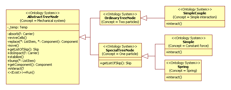
Figure 6. Concrete classes diagram

We consider model of two particles. The resolution of the model is λ= 10, μ = 1, τ = 10. Two particles with masses m1 = 2 g (1 Skip) and m2 = 1 g (no Skip - empty list) interact so that the repulsive force is independent of distance and is F = τ²/(μλ) × F’ = 10²/(1×10) × 1 = 10 dynes (use packet include 2 acts of interaction, the minimum packet that does not violate the integrity of the quantum of existence of the system). These values are chosen because they define the minimal interaction model.

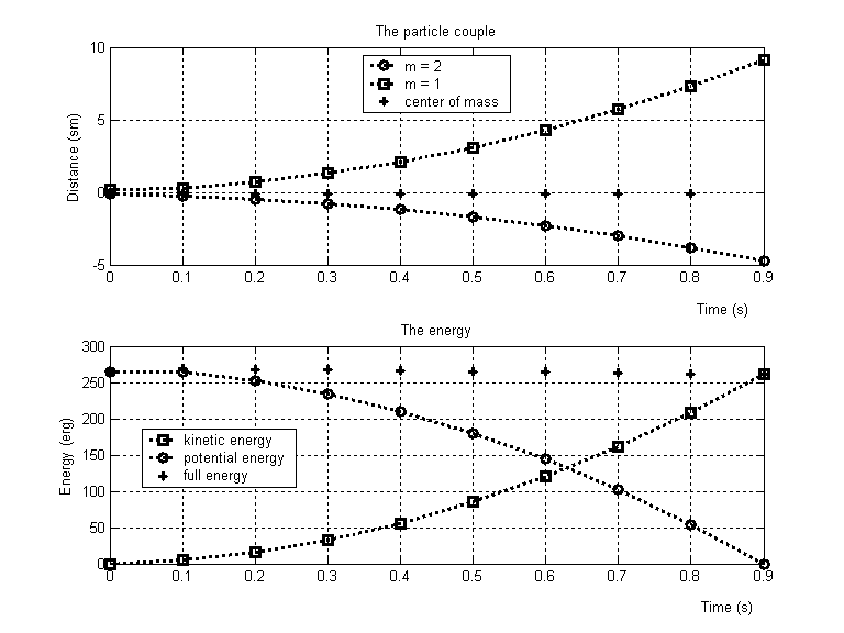
Figure 7. The graph of the motion of a pair of particles and the change in the potential, kinetic, and total energy of the system

In this experiment, the laws of conservation of momentum and energy for a closed system were verified. At the initial instant, the particles are at rest. The center of mass is at the origin of the coordinate system, the particle m1 at the point x1 = -0.1, the particle m2 at the point x2 = 0.2. Figure 7 shows the graphs of the motion of both particles and the center of inertia r = (m1x1 + m2x2) / (m1 + m2) (marked with crosses).
The lower part of the figure shows the graphs of potential (circle), kinetic (square) and total (cross) energy. The zero of the potential energy is chosen at infinity (13.6 cm at t = 0.9 sec). Potential and kinetic energy was measured by a direct method; for this, the simulation method was used. It should pay attention to reducing the total energy of the system. This is an analog of computational (countable) viscosity in numerical methods.

The simulation model in C++ code:

AppBaseClasses.h, AppBaseClasses.cpp
IntermediateLevel.h, IntermediateLevel.cpp
Models.h, Models.cpp
TreeRoot.h, TreeRoot.cpp (see Using)

Conclusion

In this section considered object model of classical mechanic motion in discrete space-time. Along with the models considered above, other models were also studied. We mention the most interesting of them: a plane shock wave in a solid, the motion of a metal chain, the destruction of a freely falling liquid stream, photonic nanojets, and a number of problems in the theory of impact. The simulation model was compared with a numerical methods such as the particle-in-cell (PIC, Harlow) method and the molecular dynamics method. A comparative analysis showed similarity and difference into approaches. The simulation model require more detail model of object under study but allow use constructions of molecular dynamics method as simplifications, for example, Lennard–Jones potential.The simulation model is more relevant model but require larger calculation resource. It must use if needful understand detail of physical process.
In our opinion, the above results allow us to state that the proposed model of mechanical motion adequately describes mechanical processes.

References

1. Gurianov V.I. Models of constructive physics in the classical mechanics of a point particle. // Mathematical models and their applications: Sat. sci. tr. Issue. 15. - Cheboksary: Publishing house Chuvash. Univ., 2013. - P. 148-159.
2. Gurianov V.I. Dynamics, Levy’s theory and the inertial mass // Mathematical models and their applications: Sat. sci. tr. Issue. 18. - Cheboksary: Publishing house Chuvash. Univ., 2016. - P. 221-231.
3. Gurianov V.I. Verification of discrete model of mechanical motion // Mathematical models and their applications: Sat. sci. tr. Issue. 19. - Cheboksary: Publishing house Chuvash. Univ., 2017. - P. 97-105.
4. Ozhigov Yu.I. Constructive physics. - SRC “Regular and chaotic dynamics”, 2010. - 440 p.
5. Structure and Interpretation of Classical Mechanics By Gerald Jay Sussman and Jack Wisdom. Also, see project on GitHub.
6. Website E. Fredkin on Digital Philosophy, URL: http://www.digitalphilosophy.org/
7. Vstovsky G.V. Elements of Information Physics. Moscow: RIC MGIU, 2002. - 257 p.
8. Vyaltsev A.N., Discrete space-time. Ed. 3rd, stereotyped. - M .: KomKniga, 2007. - 400 p.
9. Stephen Wolfram. A Class of Models with the Potential to Represent Fundamental Physics, URL: https://arxiv.org/abs/2004.08210
10. Gerard ‘t Hooft. The Cellular Automaton Interpretation of Quantum Mechanics, URL: https://link.springer.com/book/10.1007/978-3-319-41285-6