Time dilation

Module mms.experiment1 is simulated kinematic relativistic effects.

1. Experiment description

Estimated calculation for \(\pi ^+\) meson (pion):
Time we measure in metre of light time, i.e. \(3.335640 \times 10^{-9}\) seconds.
Lifetime is \( \tau_{0} = 2.6 \times 10^{-8} \) seconds or 7.8 metres of light time.
\(\beta = v/c = 0.5 \).
Moving pion has a longer decay time \( \tau = \frac{\tau_{0}}{\sqrt{1 -\beta ^2 }} = 3.0 \times 10 ^{-8}\) seconds or 9.0 metres of light time.
Distance \( d = c \times \beta \times \tau = 4.5 \) metres,
i.e. we must consider grid 10 x 10.

Parameters of experiment:
count_tick= 8, size_tick= 10
Particle_velosety= 5 ,i.e v/c = 0.5
Time count = 80
nu_t = 10.0 , nu_x = 10.0 , nu_m = 1.0
mass = 1 , lightVel = 1.0

2. Results of experiment

In table is depicted result of simulation.

Trajectory of particle and time of the particle
+----+-----+-----+------+------+-----+
| Tw |  x  |  t  |  ta  | err% |  tp |
+----+-----+-----+------+------+-----+
| 0  | 0.0 | 0.0 | 0.0  | 0.0  | 0.0 |
| 1  | 0.5 | 1.2 | 1.12 | 7.33 | 1.0 |
| 2  | 1.0 | 2.3 | 2.24 | 2.86 | 2.0 |
| 3  | 1.5 | 3.4 | 3.35 | 1.37 | 3.0 |
| 4  | 2.0 | 4.5 | 4.47 | 0.62 | 4.0 |
| 5  | 2.5 | 5.6 | 5.59 | 0.18 | 5.0 |
| 6  | 3.0 | 6.8 | 6.71 | 1.37 | 6.0 |
| 7  | 3.5 | 7.9 | 7.83 | 0.94 | 7.0 |
+----+-----+-----+------+------+-----+

Column Tw is the number of tick of model time. Column x - is the coordinate of the particle in moment Tw. Column tp is the time of the particle. We can observe dilation of time. In the particle, tp units of time elapse, but, in the rest frame of reference t units of time are registered . Column ta is analytic calculation to formula \(ta = \sqrt{s^2+x^2}\) . Value ta compare with t

\[\begin{align*} \epsilon = \bigl| \frac{t_{a} - t}{t_{a}} \bigr| \times 100 % \\ \end{align*}\]

It is column err%.

This result is depicted in Fig.1. Black “o” is the result of the measurement. The red line is analytical value.

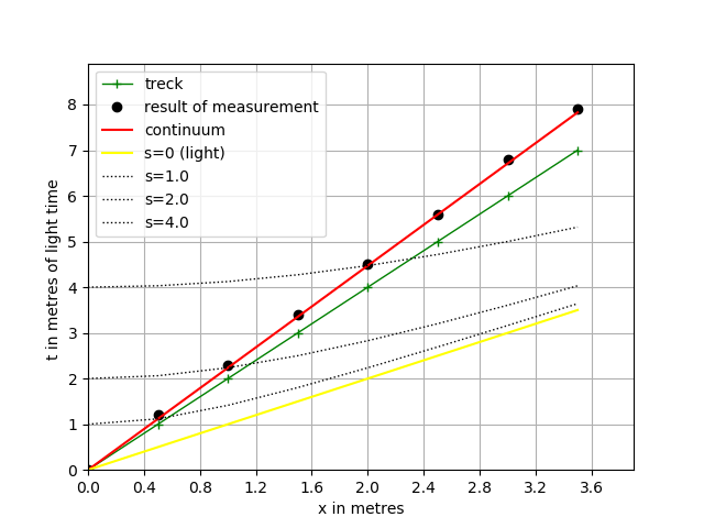
Figure 1. Minkowski spacetime diagram for \(\beta = 0.5\)

We processing of data and calculate of incline k (green line)

Experimental error of measurement t is  0.05
Point couple method (d=4)
0 20 45 2.25
1 20 44 2.2
2 20 45 2.25
3 20 45 2.25
Couple count = 4
Measurement incline k_ar= 2.24
k_ar = 2.24 +/- 0.012

Analytical incline k_an= 2.24, k_err%= 0.12  

In case of small velocity, plot depicted in Fig.2.
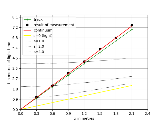
Figure 2. Minkowski spacetime diagram for \(\beta = 0.3 \)

3. Description of experiment1 modul

Class “FreeMotion”

Description: the class is a simulation model
Bases: mms.Composite
def __init__(self, size_tick, count_tick, particle_velosety, observer)

Name	Type	Description
size_tick	int	size of time tact
count_tick	int	count of tacts
particle_velosety	int	inicial speed particle
observer	Table instance	Detector and recorder

Operations:

def interaction(self, car) Description: none interaction Parameters: “car” is “Currer” instance

Class “OriginalToolkit”

Description: new procedures join to processor of data Bases: ResacherInstruments.DataProcessing
def __init__(self, observer,particle_velosety, sizeTick, countTick)

Name	Type	Description
observer	Table instance	Detector and recorder
particle_velosety	int	initial speed particle
size_tick	int	size of time tact
count_tick	int	count of tacts

Operations:

def incline(self)
Description: incline k calculate and error
Parameters: None

Algorithm:
The analytical value of incline \(k_{an}\) can deduce from the formula of the invariant interval
\( s^2 = c^2t^2 - x^2 \)
Let \(t’\) be fix moment of time then distance be \(x = vt’ \).
We have \(s = ct’ \) if \(x = 0 \).
We obtain
\( ct = \sqrt{s^2 + x^2} = \sqrt{(cx/v)^2 + x^2} = x \sqrt{1 + c^2/v^2} \) .
The result is
\( a_{an} = \sqrt{1 + c^2/v^2} \)

The experiment data processing is
\( \Delta t_{i} = t_{i} - t_{i-4} \)
\( \Delta x_{i} = x_{i} - x_{i-4} \)
\( k_{ar} = \frac{1}{N}\sum_{i=4}^{n} \Delta t_{i} / \Delta x_{i} \),
wher N is count of couples.

The standard deviation is
\( sk_{ar} = \sqrt{\operatorname {Var}(k_{ar}) / (N-1)} \), where \(\operatorname {Var}(k_{ar}) \) is variance and N is count of pair. The confidence interval is
\( dk_{ar} = sk_{ar}/\sqrt{N} \)

Then
\( k_{ar} = k_{ar} \pm dk_{ar} \)

Class “OriginalPrint”

Description: rewrite procedure xtPrintPrettyTable Bases: print_results.TablePrint