Velocity, momentum, and energy

Module experiment2.py simulated dynamic relativistic effects.

1. Experiment description

Let us consider motion of charge q in constant electric field \( \mathcal{E} \). Motion equation is

\begin{equation} \frac{dp}{dt} = q \mathcal{E} ,\ \end{equation}

where \(p\) is particle momentum, \( q \mathcal{E} \) is force.
Initial condition is \(x = 0, p = 0\) in moment \(t = 0\).
If \(t > z = m_{0}c/q \mathcal{E} \) then appear relativistic effects.
References: Charles Kittel, Walter D.Knight, Malvin A. Ruderman, Mechanics. Berkeley physics course. Vol.1, McGraw-Hill book company. 1965

We find dependence

• particle coordinate x from time t
• particle velocity v from momentum p
• particle energy E from momentum p.

Estimated calculation for electron:
\(m_{0} = 9.1 \times 10^{-31}\) kg, \(q = 1.602 \times 10^{-19}\) C
We consider simple case when \(\mu = 1\) (Skip list is NULL) and \(\iota = 1\) (one act of interaction in tick),
then
nu_m = 1.1e+30, nu_t = 3.0e+09
f = 2.7e-23 N, \( \mathcal{E} \) = 1.7e-04 V/m,
z = 10.0 s, d = 4.14 m

We will be calculated motition in \(c = 1, m_{0} = 1\) units. We introduce new variable \(p’ = p/(m_{0}c)\). If we replace \(p\) by \(m_{0}c p\) in motion equation, we obtain

\begin{equation} \frac{dp}{dt} = \frac{q \mathcal{E}}{m_{0}c}
\end{equation}

and \(f = 0.1, \nu_{t} = 10, \nu_{x} = 10\)

Variable values:
count_tick= 8, size_tick= 10
particle_velosety = 0 (initial velocity)
nu_t = 10.0 , nu_x = 10.0 , nu_m = 1.0
mass = 1 , light_vel = 1.0

With this resolution, you can perform 8 clock cycles of the system (if Tw = 9 then an error typical of relativistic models arises, which can be called “synchronization failure”).

2. Results of experiment

The results of the experiment are presented in Table 1. It is the trajectory of the particle.

Analytical (xa, pa, va) and numerical (xe) solution
+----+-----+-----+------+------+------+------+-----+------+
| Tw |  t  |  x  |  xa  |  xe  |  p   |  pa  |  v  |  va  |
+----+-----+-----+------+------+------+------+-----+------+
| 0  | 0.0 | 0.0 | 0.0  | 0.0  | 0.0  | 0.0  | 0.0 | 0.0  |
| 1  | 1.1 | 0.1 | 0.06 | 0.12 | 0.11 | 0.11 | 0.0 | 0.11 |
| 2  | 2.1 | 0.3 | 0.22 | 0.33 | 0.21 | 0.21 | 0.0 | 0.21 |
| 3  | 3.1 | 0.6 | 0.47 | 0.62 | 0.31 | 0.31 | 0.0 | 0.3  |
| 4  | 4.2 | 1.0 | 0.85 | 1.05 | 0.42 | 0.42 | 0.0 | 0.39 |
| 5  | 5.3 | 1.5 | 1.32 | 1.56 | 0.53 | 0.53 | 0.0 | 0.47 |
| 6  | 6.4 | 2.1 | 1.87 | 2.16 | 0.64 | 0.64 | 1.0 | 0.54 |
| 7  | 7.6 | 2.8 | 2.56 | 2.88 | 0.76 | 0.76 | 1.0 | 0.61 |
| 8  | 8.8 | 3.6 | 3.32 | 3.67 | 0.88 | 0.88 | 1.0 | 0.66 |
+----+-----+-----+------+------+------+------+-----+------+

Values t,x,p, and v are measurement data, values xa, pa, va are analitical solution (see class “originalToolkit”), xe - numerical solution.
Following is the plot of the trajectory (Fig.1).
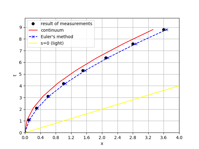
Figure 1. Motion plot

The data are presented so that speed and energy can be considered as functions of the momentum.

Velocity and energy of the particle as a function of momentum  
+----+------+------+------+--------+------+------+--------+
| Tw |  p   |  v   |  va  | v,err% |  E   |  Ea  | E,err% |
+----+------+------+------+--------+------+------+--------+
| 0  | 0.0  | 0.0  | 0.0  |  0.0   | 1.0  | 1.0  |  0.0   |
| 1  | 0.11 | 0.09 | 0.11 | 16.86  | 1.01 | 1.01 |  0.39  |
| 2  | 0.21 | 0.2  | 0.21 |  2.68  | 1.03 | 1.02 |  0.8   |
| 3  | 0.31 | 0.3  | 0.3  |  1.32  | 1.06 | 1.05 |  1.25  |
| 4  | 0.42 | 0.36 | 0.39 |  6.09  | 1.1  | 1.08 |  1.42  |
| 5  | 0.53 | 0.45 | 0.47 |  2.94  | 1.15 | 1.13 |  1.61  |
| 6  | 0.64 | 0.55 | 0.54 |  1.19  | 1.21 | 1.19 |  1.91  |
| 7  | 0.76 | 0.58 | 0.61 |  3.59  | 1.28 | 1.26 |  1.91  |
| 8  | 0.88 | 0.67 | 0.66 |  0.91  | 1.36 | 1.33 |  2.1   |
+----+------+------+------+--------+------+------+--------+

The following notation is introduced in this table: Tw is the system time step number, p is the measured pulse, v is the measured speed, va is the exact value of the speed, v, err% is the relative error of the speed measurement in%, E is the measured energy, Ea is the exact energy value, E, err% - the relative error of the energy measurement in %.
The plot of the dependence of speed on momentum is shown in Fig. 2.

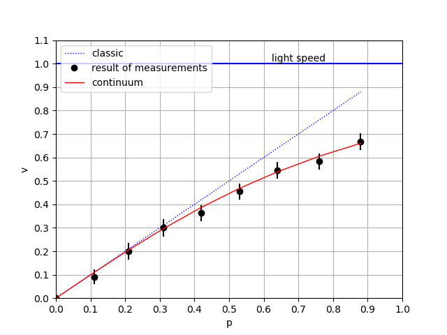
Figure 2. Velocity as function of momentum

Points are measurement data, a continuous line is an analytical curved. The dash line is a numerical solution (Euler’s method). For clarity, a plot of the dependence of speed on momentum for the classical case is also given (straight line).
The plot of the dependence of energy on momentum is presented in Fig. 3.

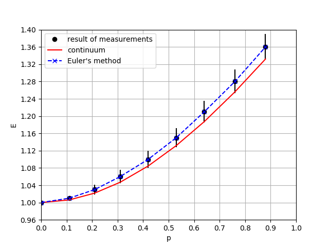
Figure 3. Energy as function of momentum

Points are measurement data. The dash line is numerical solution (Euler’s method). The continuous line is an analytical curved and compute on formula (see operation engCalculation of class mms.ResacherInstruments.DataProcessing)

\[\begin{equation} E = \sqrt{m_{0}^2c^4 + p^2c^2 } \\ \end{equation}\]

Formula \(E_{0} = m_{0}c^2\) can output from follow. Let particle be rest and force act to its. Then the particle has start of motion with delay \(\tau_{d} \)

\[\begin{equation} \tau_{d} = \tau_{R} \frac{\mu}{\iota} \\ \end{equation}\]

We get \(\mu\) and multiplying both sides by \( c^2/\nu_{m} \)

\[\begin{equation} c^2 \frac{\mu}{\nu_{m}} = c^2 \frac{1}{\nu_{m}} \times \frac{\tau_{d} \iota}{\tau_{R} } \\ \end{equation}\]

We get

\[\begin{align*} c^2 m &= c^2 \frac{1}{\nu_{m}} \times \frac{\tau_{d}}{\tau_{R}} \times \iota \\ &= c^2 \frac{1}{\nu_{m}} \times \frac{\tau_{d} }{\tau_{R} } \times \nu_{m} \frac{\tau_{R}^2}{\nu_{t}} \frac {f}{c} \\ &= c \tau_{d} \frac{\tau_{R}}{\nu_{t}} f \\ &= \tau_{d} \times c \Delta t f \\ \end{align*}\]

Combination of right side has dimension of work and we may by \(E_{0}\) denote string \(\tau_{d} c \Delta t f \).
Thus, the rest energy is the result of a delay in the start of particle motion.

3. Description of experiment2 modul

Class “SimpleIteraction”

Description: The class is a simulation model
Bases: mms.Composite
def __init__(self, size_tick, count_tick, particle_velosety, observer)

Name	Type	Description
size_tick	int	size of time tact
count_tick	int	count of tacts
particle_velosety	int	inicial speed particle
observer	Table instance	Detector and recorder

Operations:

def interaction(self, car)
Description: action of electric field
Parameters: “car” is “Currer” instance

Class “OriginalToolkit”

Description: new procedures join to processor of data
Bases: resacher_instruments.DataProcessing
def __init__(self, observer,particle_velosety, sizeTick, countTick)

Name	Type	Description
observer	Table instance	Detector and recorder
particle_velosety	int	initial speed particle
size_tick	int	size of time tact
count_tick	int	count of tacts

Attributes:

Name	Type	Description
xa_track	int array	x, analitical solution
xn_track	int array	x, numerical solution
pa	int array	momentum, analitical solution
va	int array	velocity, analitical solution
vn	int array	velocity, numerical solution
en	int array	energy, numerical solution

Operations:

def anl_solution(self)
Description: accurate x (analytical formula)
Parameters: None

Algorithm:

\[\begin{align*} &x = \frac{m_{0}c^2}{q \mathcal{E}} \Big( \sqrt{ 1 + (q \mathcal{E} t / m_{0}c)^2 } -1 \Big) \\ &v = c \sqrt{\frac{(q \mathcal{E} t/m_{0}c)^2}{1+(q \mathcal{E} t/m_{0}c)^2} } \\ \end{align*}\]

References: Charles Kittel, Walter D.Knight, Malvin A. Ruderman, Mechanics. Berkeley physics course. Vol.1, McGraw-Hill book company. 1965

def num_solution(self)
Description: numerical solution of motion differential equation (Euler’s method)
Parameters: None

Algorithm:

\[\begin{align*} &p_{i} = p_{i-1} + q \mathcal{E} \Delta t \\ &v_{i} = \frac{p_{i}} {\sqrt{m_{0}^2 + p_{i}^2 / c^2 } }\\ &x_{i} = x_{i-1} + v_{i} \Delta t \\ &e_{i} = e_{i-1} + q \mathcal{E} \Delta x \\ \end{align*}\]

where \(p_{0} = 0\), \(v_{0} = 0\), \(e_{0} = m_{0}c^2\).

Value \(x_{i}\) write to array xn_track, value \(v_{i}\) write to array vn, value \(e_{i}\) write to array en.