Analysis model

In UML2 SP, a simulation model described as an ontology. Classes are considered as the Minsky frames. The language details view on-site https://vgurianov.github.io/uml-sp/

1. Ontology of the Special Relativity Theory

Semantic net definition.
Classical mechanics concepts can view here.
Concepts in relativistic mechanics are similar to the concepts of classical mechanics, but there are differences. It is a synchronization rule of time of a mechanical system and local time of cells.
The main concepts are Physical space-time, Cell of space, Interval of time, Local Time (it is attribute frame ListItem) , and Synchronization (fig.1).

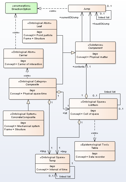Fig1 Figure 1. Ontology of Special Relativity Theory

Also, see
Full diagram
Pseudo code C++

2. Realization of use case “Run”

Use case “Run” realization is depicted in Fig.2.
Fig2
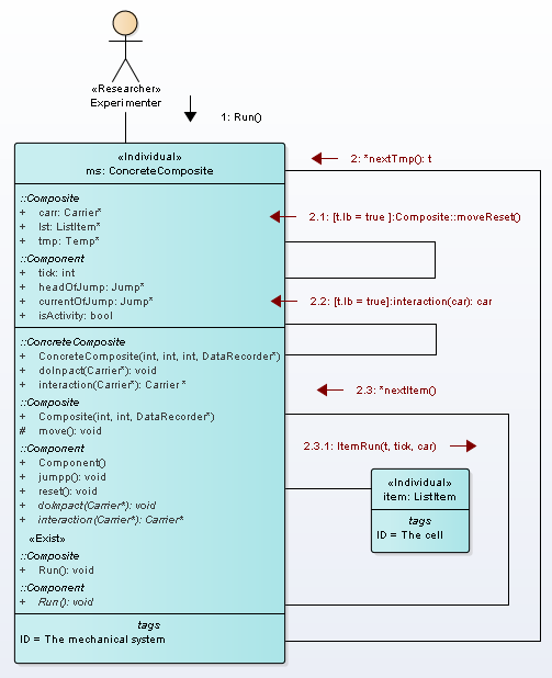
Figure 2. Communication diagram of operation “Run”

The operation Run() has the base cycle on a linked list tmp. For each node t, there executed cycle on linked list lst and each node item get message itemRun().
If node t has t.lb = true then it is called “bearing” moment of time. Nodes number between bearing moments is called resolution of tick of time (\(\tau_{R} \)). Variable tick is the count of “bearing” moments (Tw).
If node t is bearing moment then there executed operation moveReset() and interaction().

void Run() {
//t=0 is singular point
tick = 0;
Temp *t; t = tmp;
ListItem *item; item = lst;
Carrier *car; car = interaction(car);
item->ItemRun(t, tick, car);

t = t->next;
  while (t != NULL) {

    if (t->lb) {
      tick = tick + 1;
      moveReset();
      car = interaction(car);
    };
                
    item = lst;
    while (item != NULL) {
      item->ItemRun(t,tick, car);
      item = item->right;
    };

  t = t->next;
  };
} 

3. Spacetime model

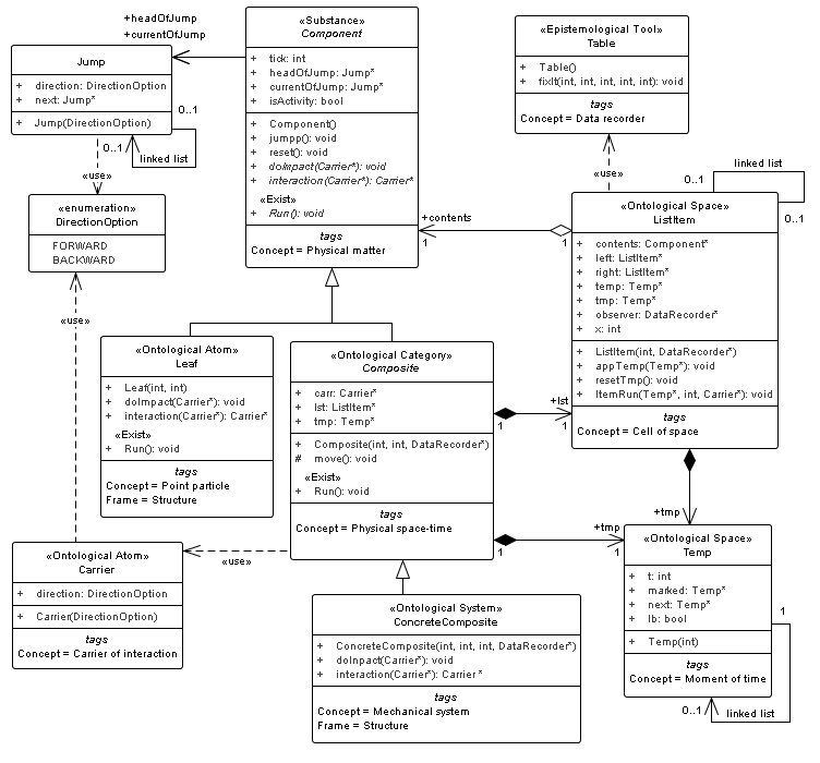
We propose the following model of Minkowski spacetime (Fig.3).
“Composite” class is a model of a physical spacetime. We will view the one-dimension space. Physical space is linked list, where “lst” attribute is base of space (In the general case, “headOfList” attribute is base of space, and “tailOfList” is the anchor point and specify the direction in the physical space). Attribute “tmp” is a one-direction linked list and it is a model of physical time. Attribute “tmp” is an instance of class Temp.
Class “ListItem” is a model of a physical space cell. The cell has a local time; it is “tmp” attribute.
The time of “Composite” class and the time “ListItem” class must be synchronized.
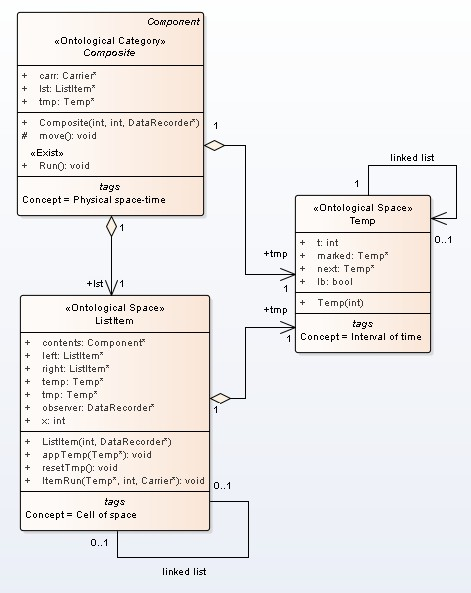Fig3 Figure 3. Minkowski spacetime model

The synchronization mechanism is the following process. Operation “Run” of class Composite has the cycle by linked list “tmp”. For each node tt of linked list “tmp” sent message runItem(tt) to all cells of space (Fig.4).
Fig4
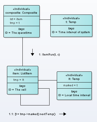
Figure 4. Communication process of synchronization

In procedure runItem(tt), tt compared with attribute “marked” of current node of “tmp” (lt on Fig.4). If tt equals “marked” then linked list “tmp” shift to next node (operation nextTemp() on Fig.4). This is jump (tick) of the local time of the cell. If the cell has the particle then the time of particle also makes shift (operation Run() on Fig.4).

void ItemRun(Temp *tt, int tGlob, Carrier *c) {
  if (tmp != NULL) {
    if (tt == tmp->marked) {
      // ---- some activity  ----
      };
    tmp = tmp->next;  // time shift in cell
    };
  };
}

Both Newton’s time and time of special relativity has the same synchronization mechanism but different rule of define “marked” label. In Newton’s mechanics, the time of “Composite” class and the time “ListItem” class has the same lengths of linked list “temp” and label “marked” has the same number with the number of node “temp”.
Time of special relativity has following rule. We take more details grid. Let size be resolution of one-time tact then k x size is length list tmp. Each size node tmp is marked as lb = true; it is “bearing” node.
Further, cells mark as

Temp *tt; ListItem *ll; int s,t,x; Temp *st;
tt = tmp;
while (tt != NULL) {
  if (tt->lb) { // It is "bearing" moment of time
    ll = lst;
    while (ll != NULL) {
      s = tt->t; x = ll->x;
      t = sqrt(s*s + x*x); //use ceil,floor
      if (t<size) {
        st = tmp;
	for (int i = 0; i < t; i++) st = st->next;
	ll->appTemp(st);
      };
      ll = ll->right;
    };
  };
tt = tt->next;
};

i.e. used formula is \( ct = \sqrt{s^2 + x^2} \).
The operation appTemp(st) create a new node of type Temp in cell and mark it as st (see Fig.5). Fig5
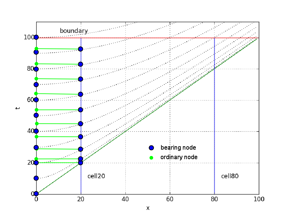
Figure 5. Example of linked list tmp for cells 20 and 80

If a reference frame has uniform translatory motion then base of space has shift. Let V be velocity a reference frame then formula \( ct = \sqrt{s^2 + (Vs -x)^2} \) define the rule of marking.

4. Mechanical motion and interaction

If local time has shift and cell has a particle then possible motion particle and interaction.
Mechanical motion and interaction are depicted in fig.6.
Fig6
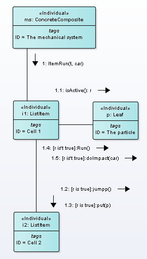
Figure 6. Mechanical motion and interaction

In Pseudocode, we have

void ItemRun(Temp *tt, int tGlob, Carrier *c) {
  if (tmp != NULL) {
    if (tt == tmp->marked) {
      if (contents != NULL) {// here particle
        if (contents->isActive) {
	  contents->jumpp();  // shift list Jump
	  oneJump(); // we move particle to the next cell
	} else {
	  contents->Run();  // time shift in particle
	  // Data write to table
	  observer->fixIt(tGlob, tt->t, x, tt->t, contents->tick);
	  contents->doImpact(c); // interaction
	  observer.detect(tGlob,c); // observe act of interaction
	};
      };
    tmp = tmp->next;  // time shift in cell
    };
  };
}

If the particle is active then the particle removes from cell 1 and place in cell 2. If the particle isn’t active then particle time has shift and the particle has interaction.
Let \(\tau_{R}\) be the resolution of tick of time and \( j \) the list length Jump.
The particle may not have a velocity of more than light speed as count jumps are not more than \( \tau_{R} \) even if \( j > \tau_{R} \). If \( j = \tau_{R} \) then particle time is stop and interaction is inpossible.
If j = 0 then time and interaction are as in classical mechanics. If \( 0 < j < \tau_{R} \) then particle time is slows down and intensity of interaction falls.

5. Measurements

All epistemology entities have standard types (int, bool, and itc.).
We define the unprimed system to follow.

Space cells marked numbers from 0 to Nmax. It is variable x class ItemList.
Time interval marked number from 0 to Nmax. It is variable t class Temp.
Counter of bearing (abutting) node (lb = true) is variable “tick”.
In all cells put detector of location and interaction. It is the variable “observer” of the class Table.

We define the time of particle (the primed system) as the variable “tick” the class Component.

Operation of measurement is depicted in Fig.7
Fig7
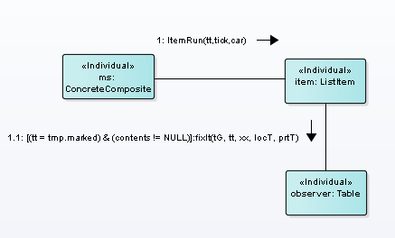
Figure 7. The measurement

Message fixIt() send if cell isn’t empty and tt = tmp.lb. Operation fixIt() write x,t, and other variable to table.

The main measurement is count. The absolute error of measurement then is 0.5.
A unit of measurement is “thing” or “piece”. A dimensional unit is a dimensionless quantity.
This system of measurement we call “natural” units, SI and CGS is called “standard” units.
Let \(\tau\) be the time, \(\rho\) distance, and \(\mu \) mass in natural units.
By \(\tau_{R} \) denote the resolution of tick of time.
Then, time \(t\), distance \(d\), and mass in standard units calculated as

\[\begin{align} &t = \frac{\tau}{\nu_{t}} , ~~ dim~ \nu_{t} = T^{-1} , \\ &d = \frac{\rho}{\nu_{x}} , ~~ dim~\nu_{x} = L^{-1} , \\ &m = \frac{\mu}{\nu_{m}} ,~~ dim~ \nu_{m} = M^{-1} , \\ \end{align}\]

where \(\nu_{t}, \nu_{x}, \nu_{m} \) are the coefficients of the conversion time, distance, and mass.
Kinematics.
Velocity will measure in ticks:

\[\begin{equation} \beta = \frac{v}{c} = \frac{\rho}{k\tau_{R}} ,\\ \end{equation}\]

where k is count tacts, \(\rho\) is traveled distance.
Dynamics.
Let \(\iota_{i} \) be the number of interaction acts in tick i (interaction intensity).
Force f is

\[\begin{equation} \label{A} f_{i}/c = \frac{1}{\nu_{m}} \frac{\nu_{t}}{\tau_{R}^2} \iota_{i} \\ \end{equation}\]

The output of the formula.
Interaction \(\iota \) change list Jump and, сonsequently, particle velocity.
We have

\[\begin{equation} \Delta p / \Delta t = f \\ \end{equation}\]

We get

\[\begin{align*} \Delta p / \Delta t &= \frac{1}{\Delta t} \biggl( \frac{m_{0}v_{i}}{\sqrt{1-\beta_{i}^2}}- \frac{m_{0}v_{i-1}}{\sqrt{1-\beta_{i-1}^2}} \biggr) \\ &= \frac{m_{0}c}{\Delta t} \biggl( \frac{\beta_{i}}{\sqrt{1-\beta_{i}^2}}-\frac{\beta_{i-1}}{\sqrt{1-\beta_{i-1}^2}} \biggr) \\ &= \frac{m_{0}c}{\Delta t} \biggl( \frac{\Delta\rho_{i}/\tau_{R}}{\sqrt{1-\beta_{i}^2}}- \frac{\Delta\rho_{i-1}/\tau_{R}}{\sqrt{1-\beta_{i-1}^2}} \biggr) \\ &= \frac{m_{0}c}{\tau_{R}/\nu_{t}} \biggl( \frac{\Delta\rho_{i}/\tau_{R}}{\sqrt{1-\beta_{i}^2}}- \frac{\Delta\rho_{i-1}/\tau_{R}}{\sqrt{1-\beta_{i-1}^2}} \biggr) \\ &= c\times m_{0}\frac{\nu_{t}}{\tau_{R}^2} \biggl( \frac{\Delta\rho_{i}}{\sqrt{1-\beta_{i}^2}}- \frac{\Delta\rho_{i-1}}{\sqrt{1-\beta_{i-1}^2}} \biggr) \\ &= c\times m_{0}\frac{\nu_{t}}{\tau_{R}^2} \biggl( \frac{j_{i}}{\sqrt{1-\beta_{i}^2}}-\frac{j_{i-1}}{\sqrt{1-\beta_{i-1}^2}} \biggr) \\ &= c\times m_{0}\frac{\nu_{t}}{\tau_{R}^2} (\iota/\mu)\\ &= c\times\frac{\mu}{\nu_{m}}\frac{\nu_{t}}{\tau_{R}^2} (\iota/\mu)\\ \end{align*}\]

where \(\mu \) is list length Skip, j is list length Jump.
We used substitution

\[\begin{align*} \Delta t = \frac{\tau_{R}}{\nu_{t}}, \beta = \frac{\Delta \rho}{\tau_{R}},\\ \end{align*}\]

and

\[\begin{align*} \iota/\mu = \frac{j_{i}}{\sqrt{1-\beta_{i}^2}}-\frac{j_{i-1}}{\sqrt{1-\beta_{i-1}^2}}.\\ \end{align*}\]

Finally, we obtain

\[\begin{equation} \frac{1}{\nu_{m}}\frac{\nu_{t}}{\tau_{R}^2} \times \iota = \frac{f}{c} \\ \end{equation}.\]

Dimention is

\[\begin{equation} dim ~ \frac{1}{\nu_{m}}\frac{\nu_{t}}{\tau_{R}^2} \times \iota = dim ~ \frac{f}{c} = MT^{-1} . \\ \end{equation}.\]

pymms

1. Simulation model

2. Package API